Creating a Comprehensive Date Table for Time Intelligence Analysis in R

lubridate

stringi

zoo

Time Intelligence

Creating comprehesive datetable feilds in R with the {stringi}, {zoo} and {lubridate} packages

Author

’Kolade Gracious

Published

September 29, 2023

Creating a Comprehensive Date Table for Time Intelligence Analysis in R Formulating comprehensive datetime fields in R with the {stringi}, {zoo} and {lubridate} package

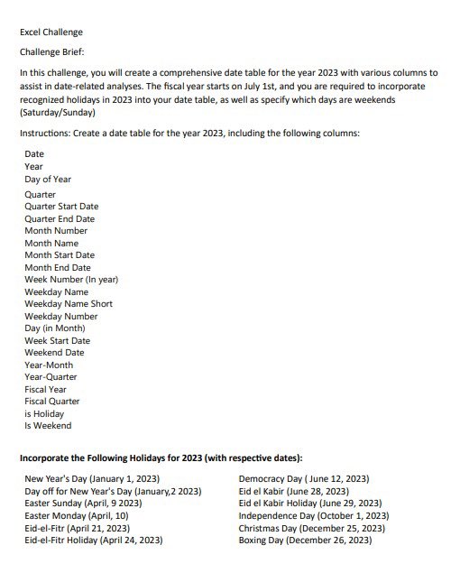
I created this post as a direct response to Malcom Okonkwo’s twitter post challenging r-lang users to create a comprehensive date table for the year 2023 in R. He solved the challenge in SQL and had quoted another post completing the same challenge using Microsoft Excel. I decided to complete this task in R.

I mean, why not? After all, R’s flexibility with datetime manipulation is notoriously underrated.

Here’s a picture of the challenge prompt.

Getting Started with the Basics

What are the task variables and problems?

Comprehensive date table needed for the year 2023
Fiscal year starts on July 1st
Recognized holidays to be incorporated into the date table as listed in the prompt
Weekends are defined as Sundays and Saturdays
Variables and corresponding observations are to be generated automatically (of course!)

Unveiling the aRtistry to Solve this Challenge

Load the required R packages needed for Time Intelligence analysis

zoo (Zeileis and Grothendieck 2005)
stringi [(Gagolewski 2022)]
lubridate [(Grolemund and Wickham 2011)]
tidyverse [(Wickham et al. 2019)]

library(tidyverse)
library(dplyr)
library(lubridate)
library(stringi)
library(zoo)

Declare fixed dependencies stored as objects first

start_date <- as.Date("2023/01/01")
end_date <- as.Date("2023/12/31")
#Fiscal year starts in July (month_number 7) every year
fiscal_start_month = 7 

##create a date matrix for recognized holidays
holiday<- as.Date(
  "2023/01/01", "2023/01/02", "2023/04/09", "2023/04/10", 
  "2023/04/21", "2023/04/24", "2023/06/12", "2023/06/28", 
  "2023/06/29", "2023/10/01", "2023/12/25", "2023/12/26"
  )

Create Date sequence automatically and store as a tibble

date_sequence <- as_tibble(seq(start_date,end_date,by = "day"))

head(date_sequence)

# A tibble: 6 × 1
  value     
  <date>    
1 2023-01-01
2 2023-01-02
3 2023-01-03
4 2023-01-04
5 2023-01-05
6 2023-01-06

Note

Generated date sequences are stored as 365 observations of the variable value. This variable name will remain unchanged throughout this post.

Mutate date_sequence to create a full date table For the sake of simplicity the sections of this stage will be discussed in three parts; Year, Quarter/Week, Fiscal Year and Weekend/Holiday wrangling

Year

datetable_year <- date_sequence %>% 
      mutate(
    ##Year
    year = year(value), #date_sequence is stored in [1] as "value"
    day_of_month = day(value),
    day_of_week = stri_datetime_fields(value)$DayOfWeek,
    day_of_week_short = format(value,"%a"),
    day_of_year = stri_datetime_fields(value)$DayOfYear,
    weekday = weekdays.Date(value),
    month = months(value),
    month_number = stri_datetime_fields(value)$Month,
    month_start_date = floor_date(as.Date(value, "%Y-%m-%d"), unit = "month"),
    month_end_date = floor_date(as.Date(value, "%Y-%m-%d"), unit = "month") 
                                                     + days_in_month(value)-1, 
    ### "-1" to make sure the exact end on the month is returned
    week_of_month = paste0("Week ", (stri_datetime_fields(value)$WeekOfMonth)),
    week_of_year =  paste0("Week ", stri_datetime_fields(value)$WeekOfYear)
      )

Now, take a look at the first part of the datetable

head(datetable_year)

# A tibble: 6 × 13
  value       year day_of_month day_of_week day_of_week_short day_of_year
  <date>     <dbl>        <int>       <int> <chr>                   <int>
1 2023-01-01  2023            1           1 Sun                         1
2 2023-01-02  2023            2           2 Mon                         2
3 2023-01-03  2023            3           3 Tue                         3
4 2023-01-04  2023            4           4 Wed                         4
5 2023-01-05  2023            5           5 Thu                         5
6 2023-01-06  2023            6           6 Fri                         6
# ℹ 7 more variables: weekday <chr>, month <chr>, month_number <int>,
#   month_start_date <date>, month_end_date <date>, week_of_month <chr>,
#   week_of_year <chr>

Quarter/Week

datetable_qtr_wk <- date_sequence %>% 
      mutate(
##Quarter/Week
        quarter = quarters.POSIXt(value),
        qtr_start_date = format(as.Date(as.yearqtr(value, format = "%Y-%m-%d")),
                                                                  "%d-%h-%Y"),
        qtr_end_date = format(as.Date(as.yearqtr(value, format = "%Y-%m-%d"), 
                                                     frac = 1), "%d-%h-%Y"),
        week_start_date = format(floor_date(as.Date(value, "%Y-%m-%d"), 
                         unit = "week", week_start = 1), "%a-%h-%y"),
        #R starts weeks on Sunday, add "week_start=1 as an arg" to coarse to Monday
        week_end_date = format(floor_date(as.Date(value, "%Y-%m-%d"), 
                                   unit = "week") + 6, "%a-%h-%y"),
        year_month = as.yearmon(value, "%m-%Y"),
        year_qrt = as.yearqtr(value, format = "%Y-%m-%d")
      )

The r chunk above create multiple qtr/wk fields using the ‘value’ variable and the functionality of the loaded R packages. A look at the second part of the date table.

head(datetable_qtr_wk)

# A tibble: 6 × 8
  value      quarter qtr_start_date qtr_end_date week_start_date week_end_date
  <date>     <chr>   <chr>          <chr>        <chr>           <chr>        
1 2023-01-01 Q1      01-Jan-2023    31-Mar-2023  Mon-Dec-22      Sat-Jan-23   
2 2023-01-02 Q1      01-Jan-2023    31-Mar-2023  Mon-Jan-23      Sat-Jan-23   
3 2023-01-03 Q1      01-Jan-2023    31-Mar-2023  Mon-Jan-23      Sat-Jan-23   
4 2023-01-04 Q1      01-Jan-2023    31-Mar-2023  Mon-Jan-23      Sat-Jan-23   
5 2023-01-05 Q1      01-Jan-2023    31-Mar-2023  Mon-Jan-23      Sat-Jan-23   
6 2023-01-06 Q1      01-Jan-2023    31-Mar-2023  Mon-Jan-23      Sat-Jan-23   
# ℹ 2 more variables: year_month <yearmon>, year_qrt <yearqtr>

Fiscal Year

datetable_fiscal_yr <- date_sequence %>% 
      mutate(
##Fiscal Year
    fiscal_year = paste0("FY-", ifelse(month(value) >= fiscal_start_month, 
                                       year(value) + 1, year(value))),
    fiscal_qrt = quarter(value, type= "year.quarter", fiscal_start = 10),
    fiscal_quarter_start_date = format(quarter(value, type= "date_first", 
                                      fiscal_start = 10), "%a-%h-%y"),
    fiscal_quarter_end_date = format(quarter(value, type= "date_last", 
                                    fiscal_start = 10), "%a-%h-%y")
      )

Now, a look at the fiscal years variables

head(datetable_fiscal_yr)

# A tibble: 6 × 5
  value      fiscal_year fiscal_qrt fiscal_quarter_start_date
  <date>     <chr>            <dbl> <chr>                    
1 2023-01-01 FY-2023          2023. Sun-Jan-23               
2 2023-01-02 FY-2023          2023. Sun-Jan-23               
3 2023-01-03 FY-2023          2023. Sun-Jan-23               
4 2023-01-04 FY-2023          2023. Sun-Jan-23               
5 2023-01-05 FY-2023          2023. Sun-Jan-23               
6 2023-01-06 FY-2023          2023. Sun-Jan-23               
# ℹ 1 more variable: fiscal_quarter_end_date <chr>

Weekend and Holiday

datetable_wknd_hol <- date_sequence %>% 
      mutate(
##Weekend and Holidays
    is_weekend = format(value, "%u") %in% c(6,7), #Saturday(6) $ Sunday(7)
    is_holiday = format(value, "%Y-%m-%d") %in% holiday
      )

head(datetable_wknd_hol)

# A tibble: 6 × 3
  value      is_weekend is_holiday
  <date>     <lgl>      <lgl>     
1 2023-01-01 TRUE       FALSE     
2 2023-01-02 FALSE      FALSE     
3 2023-01-03 FALSE      FALSE     
4 2023-01-04 FALSE      FALSE     
5 2023-01-05 FALSE      FALSE     
6 2023-01-06 FALSE      FALSE

Binding all sections together Now that all sections of the date table has been created, let’s bind them all together. This automatically merges all the code chunks above and produce a complete output.

datetable <- bind_cols(datetable_year, datetable_fiscal_yr, 
                       datetable_qtr_wk, datetable_wknd_hol,
                       .name_repair = "minimal"
                       )

Examine the dimension, column, rows and data types for the date table.

View date table

view(datetable)

Examine date table dimension

dim(datetable)

[1] 365  29

The code chunk above reveal [datetable] as a tibble with 365 rows (total days of the year) and 29 columns (feilds generated automatically).

Examine data types in date table

glimpse(datetable)

Rows: 365
Columns: 29
$ value                     <date> 2023-01-01, 2023-01-02, 2023-01-03, 2023-01…
$ year                      <dbl> 2023, 2023, 2023, 2023, 2023, 2023, 2023, 20…
$ day_of_month              <int> 1, 2, 3, 4, 5, 6, 7, 8, 9, 10, 11, 12, 13, 1…
$ day_of_week               <int> 1, 2, 3, 4, 5, 6, 7, 1, 2, 3, 4, 5, 6, 7, 1,…
$ day_of_week_short         <chr> "Sun", "Mon", "Tue", "Wed", "Thu", "Fri", "S…
$ day_of_year               <int> 1, 2, 3, 4, 5, 6, 7, 8, 9, 10, 11, 12, 13, 1…
$ weekday                   <chr> "Sunday", "Monday", "Tuesday", "Wednesday", …
$ month                     <chr> "January", "January", "January", "January", …
$ month_number              <int> 1, 1, 1, 1, 1, 1, 1, 1, 1, 1, 1, 1, 1, 1, 1,…
$ month_start_date          <date> 2023-01-01, 2023-01-01, 2023-01-01, 2023-01…
$ month_end_date            <date> 2023-01-31, 2023-01-31, 2023-01-31, 2023-01…
$ week_of_month             <chr> "Week 1", "Week 1", "Week 1", "Week 1", "Wee…
$ week_of_year              <chr> "Week 1", "Week 1", "Week 1", "Week 1", "Wee…
$ value                     <date> 2023-01-01, 2023-01-02, 2023-01-03, 2023-01…
$ fiscal_year               <chr> "FY-2023", "FY-2023", "FY-2023", "FY-2023", …
$ fiscal_qrt                <dbl> 2023.2, 2023.2, 2023.2, 2023.2, 2023.2, 2023…
$ fiscal_quarter_start_date <chr> "Sun-Jan-23", "Sun-Jan-23", "Sun-Jan-23", "S…
$ fiscal_quarter_end_date   <chr> "Fri-Mar-23", "Fri-Mar-23", "Fri-Mar-23", "F…
$ value                     <date> 2023-01-01, 2023-01-02, 2023-01-03, 2023-01…
$ quarter                   <chr> "Q1", "Q1", "Q1", "Q1", "Q1", "Q1", "Q1", "Q…
$ qtr_start_date            <chr> "01-Jan-2023", "01-Jan-2023", "01-Jan-2023",…
$ qtr_end_date              <chr> "31-Mar-2023", "31-Mar-2023", "31-Mar-2023",…
$ week_start_date           <chr> "Mon-Dec-22", "Mon-Jan-23", "Mon-Jan-23", "M…
$ week_end_date             <chr> "Sat-Jan-23", "Sat-Jan-23", "Sat-Jan-23", "S…
$ year_month                <yearmon> Jan 2023, Jan 2023, Jan 2023, Jan 2023, …
$ year_qrt                  <yearqtr> 2023 Q1, 2023 Q1, 2023 Q1, 2023 Q1, 2023…
$ value                     <date> 2023-01-01, 2023-01-02, 2023-01-03, 2023-01…
$ is_weekend                <lgl> TRUE, FALSE, FALSE, FALSE, FALSE, FALSE, TRU…
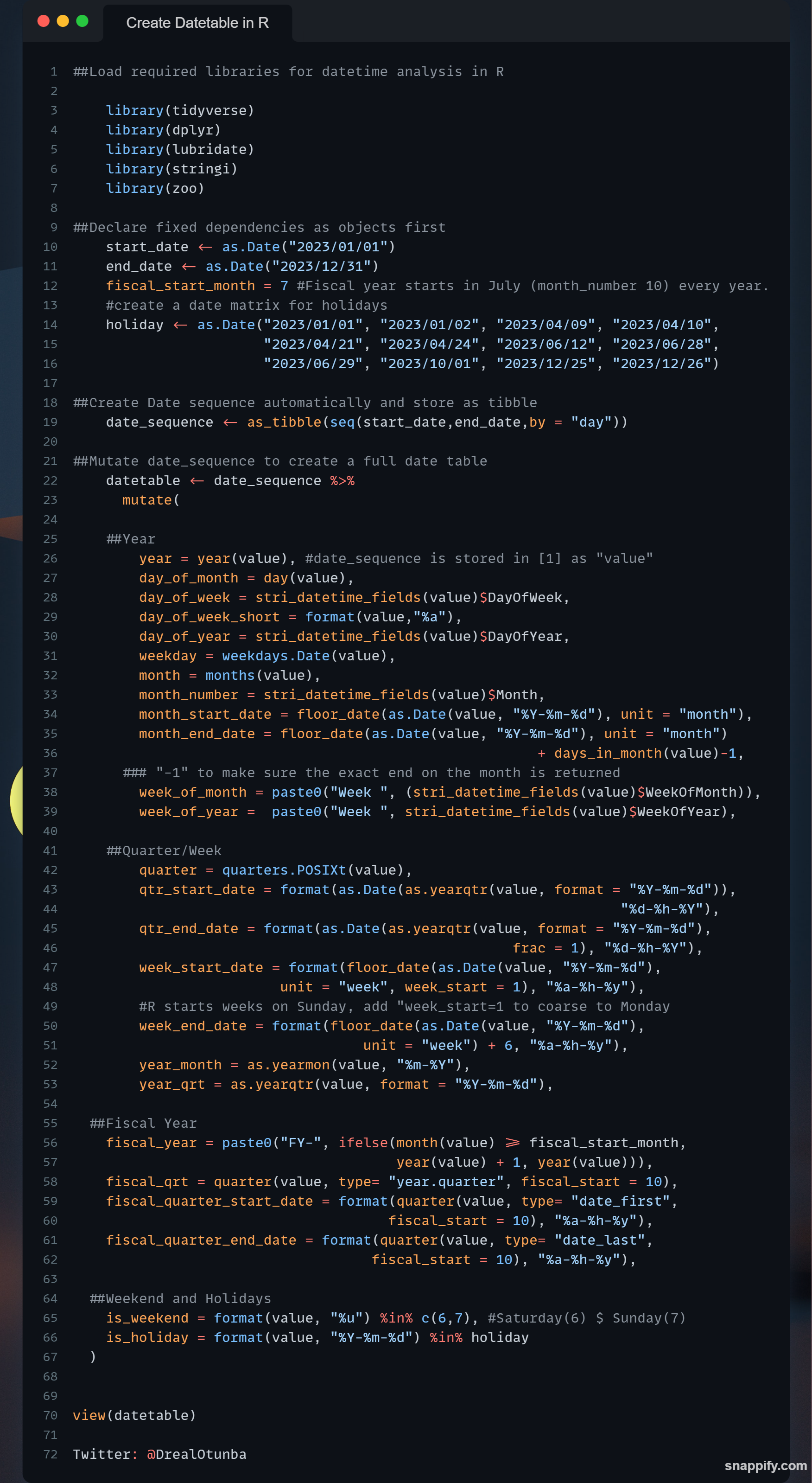
$ is_holiday                <lgl> FALSE, FALSE, FALSE, FALSE, FALSE, FALSE, FA…

Code Block

A screen grab of all r-chunk as one? Why not?

Packages Used:

Gagolewski, Marek. 2022. “Stringi: Fast and Portable Character String Processing in r” 103. https://doi.org/10.18637/jss.v103.i02.

Grolemund, Garrett, and Hadley Wickham. 2011. “Dates and Times Made Easy with Lubridate” 40. https://www.jstatsoft.org/v40/i03/.

Wickham, Hadley, Mara Averick, Jennifer Bryan, Winston Chang, Lucy D’Agostino McGowan, Romain François, Garrett Grolemund, et al. 2019. “Welcome to the Tidyverse” 4: 1686. https://doi.org/10.21105/joss.01686.

Zeileis, Achim, and Gabor Grothendieck. 2005. “Zoo: S3 Infrastructure for Regular and Irregular Time Series” 14. https://doi.org/10.18637/jss.v014.i06.